User:Thijshijsijsjss/Pen Plotting Panache/Plothatching Workflow
This is a documentation of my workflow for making multicolor crosshatching plots. It should (ultimately) be comprehensive for anyone by links and step-by-step guides, but is for now primarily written for my own future reference. This means that there are many options for each of these steps, and I will limit myself to those strategies I have found to work for me. I encourage any reader to explore different strategies! A beautiful thing about pen plotting is that every plotter (the machine) exhibits different quirks, just like any plotter (the human). It's all about engaging with, being surprised by and curiously investigating these oddities. Enjoy :)
I will make reference to several pieces of software. Notably:
- Krita, open source painting software (V5.1.5)
- Inkscape, open source vector manipulation software (V1.2)
- Some code I have written for crosshatching. Find it here on GitHub. Also, find its dedicated wiki page here
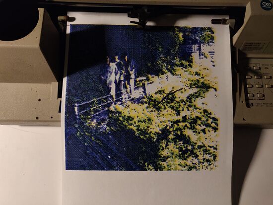
All examples shown are made with an HP7475 A3 plotter
Image selection
There's no real limit to what images can be plotted! These techniques are pretty flexible and powerful. However, still image selection seems to be one of the harder steps in this process.
Some things to keep in mind:
- Plotting takes quite a bit of time and attention. Not only the act of plotting itself, but also the preparations require a significant amount of time. Choose your current project accordingly.
- Monochrome plots are way faster than multicolor plots, both due to reduced plotting and prepping time. Additionally, the babysitting that tends to be automatic when penplotting is largely only important when switching out pens. One pen (one color) can be safely let free to plot without being babysat.
- Your selection of pens matters. Just like every plotter has its quirks, every combination of pens has its unique vibe. It's not a bad idea to take your options of pens into consideration for your choice of image.
- The crosshatching technique tends to work best for certain images:
- Images with high contrast; this will improve the level of detail that will be perceived in the final plot
- Multicolor images where the different pens will need to interact 'interestingly': nice pieces of overlap balanced with areas of one color.
- Multicolor images don't want to be very dark when plotted with a dark color for 'key'; the 'key' color will just cover everything
These final few considerations, of course, only matter if you're after a 'accurate' or specific pen plotted representation of the original image. It can be lots of fun to let yourself be surprised be the outcome of the plotter, without fretting too much what the result will be like. So take these guidelines with a grain of salt!
Image preparation
Dimensions
To avoid having to scale many layers individually later on, it's easiest to determine the size of your plot at the start. As the plotter is fastest in its horizontal axis, it is advised to orient your image in a way so that the largest dimension is the horizontal one (i.e. by rotating a portrait mode image). However, when wanting to make a plot as large as possible, this is obviously not always desired. In that case, keep bounds of 1100px by 1450px in mind (the full size of the paper in pixels according to Inkscape's default conversion).
My three most used choices for image width are:
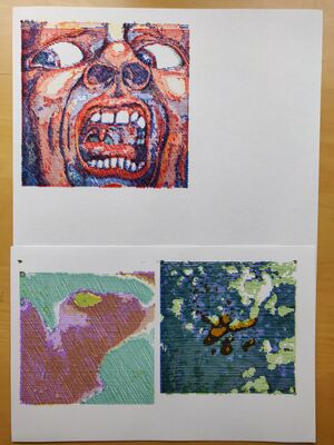
- 500px: This allows for two same width plots to be placed next to eachother on the width of the A3 plotter I have been using.
- 600px: 500px plots feel quite small. I have found 600px to be the sweet spot for compact plots that still capture quite some detail.
- 1000px: this is the about the full width of the A3 plotter I have been using.
Note that this conversion between pixels and real world measurements units is actually arbitrary. This discussion has the Inkscape default conversion in mind. Relying on this conversion saves us potentially difficult conversion problems later on, and has proven reliable between plots.
When planning to plot in a different orientation than the original image, this is the ideal time to apply the appropriate rotation
Passe Partout
Eventually, we'll need to create vector paths out of the images the crosshatching software outputs. As plotting is a lenghty step, any preparations we can do to improve the plotting time, will reduce the overall time it takes to create a plothatched image. One such improvement is the way the vector paths are traced. In Inkscape, 'Centerline (autotrace)' has the best results, by far. However, it will often (~60% of the time) crash Inkscape, in which case one has to resort to less efficient tracing methods that will typicially cause each line to be drawn from it's center (effectively adding >50% extra plotting time).
By adding a white border, a 'passe partout', around your image, Centerline (autotrace) has a better chance to succeed. In fact, borders of 100px have had a 100% success rate for me (n>200). This will NOT affect the final dimensions of your plot.
- Open your file in Krita
- Go to Image > Resize Canvas
- Add 100px to the smallest of your image's dimenstions
- Click OK
- Save image (overwrite it)
Layer separation
We will separate the different color channels and save them as individual files, so that we will be able to plothatch them individually.
- Open your file in Krita
- Change color space to CMYK
- Image > Convert Image Color Space
- Choose Model: CMYK / Alpha
- Click OK
- Separate image
- Image > Separate Image
- Click OK
- Invert all layers. For each of the layers:
- Go to a layer and press ctr+I
- Save layers 'cyan', 'yellow', 'magenta' and 'black' separately. For each of the layers:
- Toggle visibility for only one of these layers
- Save (ctr+shft+S)
- Fix opacity. For each of the new images:
- Open the image with the Windows default images app
- Three dots > Change image size
- Save image (overwrite it)
Transparancy adjustments
The previous step will typically output jpg or png images for which the transparancy mysteriously is interpreted as black. Often this is not what we want. Magically, opening an image in Windows 10's default image viewer and re-saving it (overwriting it) fixes the transparancy. This is a quick process. For other operating systems, I imagine Krita and Inkscape both support functionality to handle this.
Optionally, manual color removal
There are reasons you might want certain areas of a specific color removed before starting the hatching process. You might want this because you have certain color outcomes in mind, or because you expect this to result in more efficient plotting. In the example below, two areas of color are removed from the magenta image: first, the areas that will be black. These areas need no magenta! Second, the areas that will be yellow. In the original image, these areas are orange-y, but I'd like them to be very yellow. As I know the magenta I'll be using is quite dominant over yellow (example), we remove the area from the magenta base image. Similarly, a small chuck of blue is removed.
Hatching
This step describes the conversion of your selected and prepared image file to crosshatched layers using some Processing code. A dedicated page of this software can be found here.
First time only: downloading the script
To crosshatch your own images, you'll need to be able to compile a Processing file. For this, there are several options:
- The easiest is downloading the Processing IDE
- You can also compile from the command line
- Your favorite IDE might offer plugins for Processing language and compilation support, like this one for vscode
Next, you need to obtain the code. Again, there are several options:
- Go to https://github.com/Nyxaeroz/Crosshatching, press the button that says code, download the zip and unzip it wherever you want this project to reside on your machine.
- Moving to your desired location and use the following command in a terminal to clone the repository:
git clone https://github.com/Nyxaeroz/Crosshatching.git
Preparing script
The script uses some parameters. Crucially, you need to specify the dimensions of your image in two places.
- Open
sketch.pde - Change the variable
input_name(line 4) to match your input file's name (if this file is not located in the same folder as hachter.pde, provide the path). - Change the variables
input_width(line 11) andinput_height(line 12) to the dimensions of your file. - Change
size(W,H)(line 18) such that W and H are the width resp. height of your file.
Optional Parameters
Several parameters may be altered to achieve different results. In particular:
int nr_layers(line 6): the number of crosshatch-layers to be used.int v_line_offset(line 8): the space between two lines within one crosshatch-layerfloat blur-radius(line 9): because, often, we don't want the smallest details to appear in our crosshatch, we apply a Gaussian blur. This radius determines it's size. A size of 0 can be used to not use a blur.boolean save(line 14): the program will save the layers if and only if 'save' is set to true. Not saving would still display the image, and is useful e.g. in tweaking the parameters.
I have found that a default configuration of nr_layers=4, v_line_offset=5 and blur-radius=2 has a good success rate. I usually set save=false to try out some tweaks before setting it to true to save.
Hatching each layer
If you've followed the steps above, all images for the different color channels should be of the same dimension. This is useful, as this means preparing the script needs to be done but once (aside from choosing a different input_name of course).
For each layer, the optional parameters may be tweaked individually. By default I use the same configuration for every layer, however not uncommon exceptions include:
- using fewer layers for the Key color channel, as this layer tends to dominate the final result.
- using just one layer for big fills of on color (especially if I know I'm using markers or other wide tipped pens).
For each color channel you want to hatch:
- Set
input_name(line 4) to the corrent filename. - Tweak the optional parameters if so desired
- Run the program
- Find the output files, seperate svg layers, int a folder output_layers
- Move these layers to a new location so that they are not overwritten.
Customizations
Manual thresholds
Sometimes it is useful to manually set the threshold values for each layer. For example when aiming for specific effects, or when an image's range of values is small. Add these lines on top:
boolean use_manual_t = true;
float[] manual_t = {0.1,0.2,0.3}; // specify nr_layers many numbers
And change line 36 to:
if ( use_manual_t ) {
  output_layers[i] = create_layer( manual_t[i], my_theta );
} else {
  output_layers[i] = create_layer( my_thresh, my_theta );
}
(Similarly, one could use manual angles for each layer. I've not explored this yet, but there's some interesting potential here, e.g. in incorporating Moire Patters or playing with optical illusions).
Custom output folder
Setting custom output folder: just like the input_name (line 4) is explicitly specified, one can explicitly specify an output location. Add this line on top:
String output_folder = "MY_OUTPUT_FOLDER";
And modify line 41 to be:
beginRecord(SVG, output_folder + "/layer_" + i + ".svg");
Inkscape
Prepare document
We will prepare the document we will be working with. First, set the documents size:
- Go to File > Document Properties (Ctrl+Shift+D)
- Choose Format: A3 (or any other appropriate filesize). Note that this is primarily for the width, and not so much for the height of the paper (i.e. feeding a sheet of A4 paper in landscape mode to the plotter and plotting something from A3 settings that fits within the bounds of the A4 sheet will not cause any problems).
Next, create the layers for each color channel, and one additional layer that we'll use for importation and organization purposes. In the case of a CYMK plot:
- Open de Layers and Object tab by going to Layers > Layers and Objects (Ctrl+shift+L)
- Create 4 new layers with the dedicated button, or with Strl+Shift+N
- Rename the layers res, cyan, yellow, magenta, black (this is not strictly necessary, but useful for referencing layers within this guide, and also useful for yourself later on).
Steps for each color channel image
We will now do some preparations for each color we'll be plotting with. Confusingly, there are two notions of 'layer' here: the Inkscape 'layers', which can be thought of as folders that contain all the paths that sould be drawn with one pen. Then, there are the 'layers' of the physical world: layers of the same color that will be drawn on top of each other.
The following steps need to be taken for each color we're going to plot with, i.e. for each set of output layers we have created with the crosshatching software.
- Select the res layer
- Import all crosshatched layers of one color channel to the res folder. This is easiest by selecting them all in a file explorer and dragging them ONTO THE CANVAS AREA (note that Inkscape will crash when they are dragged onto the layers menu), but this can also be done one by one through Inkscape's import menu.
- For each imported object, you'll see a sublayer in Inkscape with an image. For each of these sublayers:
- Position it at (0,0) by selecting the Select Tool, selecting the relevant sublayer, and setting x and y fields to 0.
- Still with the Select Tool, select the image in the sublayer, and go to Trace Bitmap (Shift+Alt+B, Path>Trace Bitmap, or through the quick menu if it's still open)
- MAKE SURE SMOOTH CORNERS IS TICKED OFF
- Click Apply
- Move all paths that have been created to the appropriate Inkscape layer.
- Delete all contents from the res layer.
Alignment thingies
When plotting through Inkscape, the top-left corner of your plot is determined at the time of starting the plot, and all paths in that 'batch' are positioned relative to that origin point. This means that when plotting two paths with top-left corners at (X,Y) and (X+n,Y+m) (n,m>=0), these will be plotted at (0,0) and (n,m). In other words: the relative position is maintained when plotting multiple paths at a time.
When sending new paths to the plotter, however, this origin is redetermined. So when plotting a path with top-left corner at (X,Y) and then separately plotting a path with top-left corner at (X+n,Y+m) (n,m>=0), these will both be plotted at (0,0). In other words: the relative position is lost when plotting paths separately.
Typically, we desire the relative position to be maintained. As it is always the top-left corner that determines the position, we will add a marker -- and 'alignment thingy' -- in the same absolute position for each batch of paths we will plot.
- In Inkscape, determine the absolute position of your origin point. Let's call this (N.M)
- If you're not using a passe partout, (N,M) = (0,0)
- Otherwise, it will be different. For a passe partout of 100px both to width and height, (N,M) = (26,26)
- Select the Square Tool and draw a square of any size on any position on the canvas (typically I would do this in the res layer)
- Select the Select Tool and select the newly drwan square
- Set its parameters: x=N, y=M, w=0.1, h=0.1
- Use Right Click > Duplicate on this alignment thingy, such that you have one for each batch (typically: each layer) you'll be plotting
- Move one alingment thingy to each batch (typically: each layer).
Tip: the visible layers will be plotted top to bottom, and the paths in within each layer bottom to top. Therefore, it is advised to place the alignment thingy as the bottom path of each layer. By doing so, it immediately becomes clear if there are alignment issues.
Usually, I'd go over each layers and set their position to (0,0). This is not relevant for the actual location of the plot, but is useful when wanting to position multiple plot on the same sheet of paper. On that note:
When plotting multiple plots next to each other on one sheet of paper, the alignment thingy can be used for the appropriate offsets. E.g. when plotting two 500x500px plots side by side, the latter's alignment thingy should be offset by (-500,-500).
Optionally, scaling and rotation
Sometimes you might want to scale or scale a prepared image, e.g. in an effort to use most of your sheet of paper, or to fit multiple plots side by side.
Ideally, rotations and scaling are done in the setting dimensions step.
This is not always possible, however, e.g. if you're using the preparations of an image you've previously plotted in a different orientation. In this case, this is the time to apply these transformations.
Scaling is easy. For each layer:
- Go to Object > Transform (Ctrl+shift+M)
- Go to the scale tab
- Input the new scale
Rotation is more involved. On the surface, it is similar. For each layer:
- Go to Object > Transform (Ctr+shift+M)
- Go to the rotation tab
- Input the new rotation
HOWEVER: note that the origin of rotation is relative to the object. This means that properly aligned objects of different sizes might lose their relative positions after each rotation the same amount. Alignment thingies can be used to prevent this. Depending on your rotation, you might need to add an alignment thingy to another corner. Worst case scenario, you need to move your rotated object (or use Ctr+Z to undo).
Optionally, automated layer names
There is neat functionality within Inkscape to tell the plotter what pen to use and with what speed to plot. This can be done by giving a layer a specific name:
Pen {1,2,3,4,5,6} Speed 0
Exactly one number out of {1,2,3,4,5,6} should be chosen. For the speed, any natural number (or positive real?) can be used, but I've yet to come across a situation where I did not want to use 0 (fassst plotting).
Setting these layer names is very useful when wanting to automate a bigger plot: by naming all layers using this convention, you can plot with (in the case of my plotter) 6 pens 'at once'. This is the most reliable way of good relative alignment between layers.
Plotting
Finally, it is time to actually plot! With everything prepared, it should be smooth sailing from here. However, it is never a bad idea to keep an eye out when plotting. For starters, there might be small issues to fix (alignment issues, pens not being held correctly, paper tearing, ...) But aside from that, watching the pen plotter work is a mesmerizing victory lap for all the work you put in! It's a musical, mechanical performance that wants to be witnessed!
Tip: during plotting, you can use the 'view' button on your plotter to pause the plot and make minor adjustments to the pen and the paper alignment
You might want / need to abort a plot. For this, you must both turn off the plotter AND unplug the usb connection to your machine. Then, turn the plotter back on and replug it.
Pens
Pens are a fun step. So far, we have used the CMYK color space. However, this is just a shackle of the digital realm. In our pen selection, we can use any combination of pens we want, chosen from the continuous real world space of colors. Of course, if your goal is a true-to-screen representation of your image file, then you should use cyan-ish, magenta-ish, yellow-ish and black-ish colors.
Multiple pens
When using Inkscape's layer-to-pen functinality, or when the use of multiple pens is specified through HPGL code, it is possible to preload all pens into the carousel (in the correctly numbered spots!) and plot in one go. This is very convenient when you need to get away from the plotter. However, it is less reliable. Some issues that might occur:
- Pens not being grabbed correctly (unlikely with 'real' pen plotter pens, but it does occur for pens in custom holders)
- Alignment issues between layers (always, ALWAYS use alignment thingies)
- The carousel tends to be dirty, so your pens might pick up some different color (especially ones with a light color)
Therefore, if the situation allows for it, it is more reliable to plot different colors separately.
'Real' and custom pens
There are 'real' pens, meant for pen plotting. These tend to work nicely, but they also tend to be green (within the confines of the xpub studio). They are very friendly to use, and often provide nice results. However, they are limited in color selection and pen texture. Therefore, one might consider using their own pens. For the main wiki page on this topic, see Pen Hacking.
- One strategy is to cut open a 'real' pen so that you can load in your own.
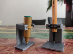
- Another strategy is to 3d print a custom holder.
- This is a GitHub repo with many stl files. The one I have tried did not work for me, however (too slim for the pen specified, or not aligned properly).
- I have made my own (specifically for stabillo 68 / 88 pens), the stl files for which can her found here on Gitea
When using a custom pen, it is crucial to align it properly heigh wise. This can be done by hand, by comparing a pen in a custom holder side by side with a 'real' pen. To make this process more reliable and less tedious, I have also made a rig for veritcal alignment. These files, too, can be found here on Gitea
Plotting through Inkscape
- Open your prepared files.
- Turn on the visibility of a layer if and only if you are planning to plot it right now
- Go to Extensions > Export > Plot
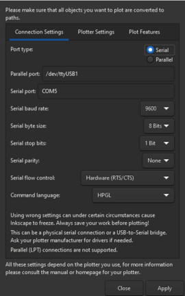
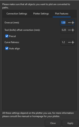
- Check the settings (see below). For my particular plotter, it is important to set Plotter Settings > Rotation to 270. For others, it is important to select Plotter SEttings > Center origin. This might require a bit of trial and error.
- Click Apply
The plotter's alignment is determined from the moment you open the Export > Plot menu. This means that, as long as you don't close this window and the paper in the plotter is not touched, the alignment will be the same. In particular: YOU CAN MAKE CHANGES TO THE FILE WITHOUT CLOSING THIS WINDOW. This includes toggling visibility. So, when plotting with multiple pens separately, keep this window open!
Tip: making use of the above observation, you can toggle the visibility for an alignment thingy only to check the alignment of your plotter.
Plotting through Chiplotle
It is possible to plot through the command line using a python environment. I have not been using this, so for now I will refer to the guide on the main pen plotter page. However, in a way this is an extension of the method described here: we can use Inkscape to export to HPGL, which is needed for plotting with Chiplotle.
Exporting HPGL
Instead of directly sending a file to the plotter through Inkscape ('directly' in so far that any conversion steps are not made explicit), we can also export to HPGL: go File > Export (Ctrl+Shift+E) and select HPGL. You might need to add a module to your Inkscape for this export option to appear. Again, I refer to the the main pen plotter page. For me, this option doesn't work. However, another way to export to HPGL is using Save As and selecting .hpgl there.
The HPGL export behave as you'd hope they'd do: they follow the exact order Inkscape would also plot in. That is, it goes through the layers from bottom to top, and objects within layer from bottom to the top. Also, pen selection automatisation using layer names is exported, too.
Setting up Chiplotle
To use Chiplotle, it needs to be setup on your machine. For this, I refer to the pypi page and the the main pen plotter page.
Sending files through Chiplotle
Navigate to the folder with your file(s) and start Chiplotle:
> Chiplotle3
It will search for connected devices. Your pen plotter should be shown. Now you can write to this plotter:
> plotter.write_file('FILENAME.hpgl')
Chiplotle will take care of many things, including the buffer size. It seems to do this well -- in cased where Inkscape wasn't able to properly export to a plotter, Chiplotle has been able to.
